Топ 5 онлайн компилятора python

Linear Algebra with Python SciPy

Linear Algebra represents linear equations and represents them with the help of matrices.

The sub-module of the SciPy library is used to perform all the functionalities related to linear equations. It takes the object to be converted into a 2-D NumPy array and then performs the task.

1. Solving a set of equations

Let us understand the working of the linalg sub-module along with the Linear equations with the help of an example:

4x+3y=123x+4y=18

Consider the above linear equations. Let us solve the equations through the function.

from scipy import linalg
import numpy
X=numpy.array(,])
Y=numpy.array(,])
print(linalg.solve(X,Y))
X.dot(linalg.solve(X,Y))-Y

In the above snippet of code, we have passed the coefficients and constant values present in the input equations through numpy.array() function.

Further, function solves the linear equations and displays the x and y value which works for that particular equation. command is used to check the output of the equations.

Output:

 ]
array(,
       ])

array(, ]) ensures that the linear equations have been solved rightly.

]: These are the x and y values used to solve the linear equations.

2. Finding the Determinants of Matrices

The method is used to find the determinant of the input matrix.

Example:

from scipy import linalg
import numpy
determinant=numpy.array(,])
linalg.det(determinant)

Output:

8.0

3. Calculating Inverse of a Matrix

The method is used to calculate the inverse of an input matrix.

Example:

from scipy import linalg
import numpy
inverse=numpy.array(,])
linalg.inv(inverse)

Output:

array(,
       ])

SciPy linalg

SciPy has very fast linear algebra capabilities as it is built using the optimized ATLAS (Automatically Tuned Linear Algebra Software), LAPACK(Linear Algebra Package) and BLAS(Basic Linear Algebra Subprograms) libraries. All of these linear algebra routines can operate on an object that can be converted into a two-dimensional array and also returns the output as a two-dimensional array.

You might wonder that numpy.linalg also provides us with functions that help to solve algebraic equations, so should we use numpy.linalg or scipy.linalg? The scipy.linalg contains all the functions that are in numpy.linalg, in addition it also has some other advanced functions that are not in numpy.linalg. Another advantage of using scipy.linalg over numpy.linalg is that it is always compiled with BLAS/LAPACK support, while for NumPy this is optional, so it’s faster as mentioned before.

Solve Linear Equations

We can use scipy.linalg.solve() to solve a linear equation, all we need to know is how to represent our equations in terms of vectors. Here is an example:

import numpy as np  
from scipy import linalg  
# We are trying to solve a linear algebra system which can be given as   
#         x + 2y - 3z = -3 
#         2x - 5y + 4z = 13  
#         5x + 4y - z = 5  
#We will find values of x,y and z for which all these equations are zero
#Also finally we will check if the values are right by substituting them
#in the equations
# Creating input array  
a = np.array(, , ])  
# Solution Array  
b = np.array(, , ])  
# Solve the linear algebra  
x = linalg.solve(a, b)  
# Print results  
print(x)  
# Checking Results  
print("\n Checking results,must be zeros")  
print(a.dot(x) - b)  

As we can see, we got three values i.e 2,-1 and 1.So for x=2,y=-1 and z=1 the above three equations are zero as shown above.

Finding a determinant of a square matrix 

The determinant is a scalar value that can be computed from the elements of a square matrix and encodes certain properties of the linear transformation described by the matrix. The determinant of a matrix A is denoted det, det A, or |A|. In SciPy, this is computed using the det() function. It takes a matrix as input and returns a scalar value.

#importing the scipy and numpy packages
from scipy import linalg
import numpy as np
 
#Declaring the numpy array
A = np.array(,,])
#Passing the values to the det function
x = linalg.det(A)
 
#printing the result
print('Determinant of \n{} \n is {}'.format(A,x))

Eigenvalues and Eigenvectors

For a square matrix(A) we can find the eigenvalues (λ) and the corresponding eigenvectors (v) of by considering the following relation

We can use scipy.linalg.eig to computes the eigenvalues and the eigenvectors for a particular matrix as shown below:

#importing the scipy and numpy packages
from scipy import linalg
import numpy as np
 
#Declaring the numpy array
A = np.array(,,])
 
#Passing the values to the eig function
values, vectors = linalg.eig(A)
 
#printing the result for eigenvalues
print(values)
 
#printing the result for eigenvectors
print(vectors)

1.6.8. Fast Fourier transforms: scipy.fftpack¶

The module computes fast Fourier transforms (FFTs)
and offers utilities to handle them. The main functions are:

• to compute the FFT
• to generate the sampling frequencies
• computes the inverse FFT, from frequency
  space to signal space

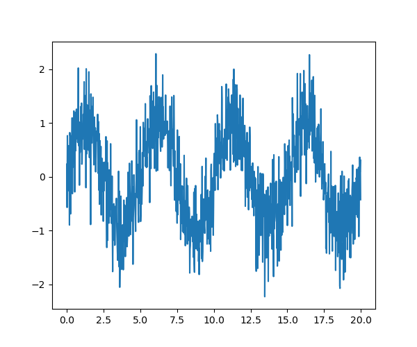
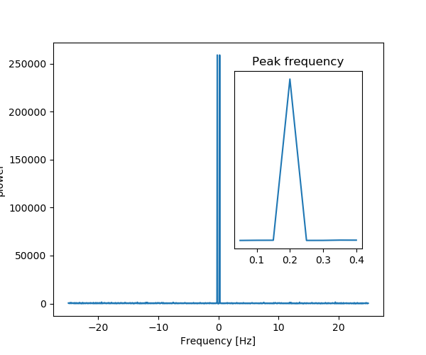
As an illustration, a (noisy) input signal (), and its FFT:

>>> from scipy import fftpack
>>> sig_fft = fftpack.fft(sig) 
>>> freqs = fftpack.fftfreq(sig.size, d=time_step) 

Signal	FFT

As the signal comes from a real function, the Fourier transform is
symmetric.

The peak signal frequency can be found with

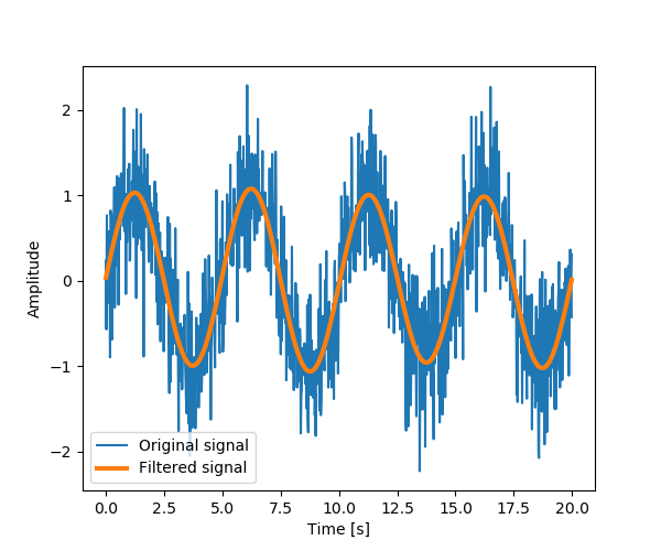
Setting the Fourrier component above this frequency to zero and inverting
the FFT with , gives a filtered signal.

Note

The code of this example can be found

numpy.fft

Numpy also has an implementation of FFT (). However,
the scipy one
should be preferred, as it uses more efficient underlying implementations.

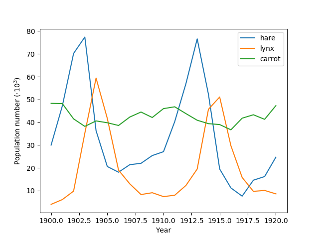
Fully worked examples:

Crude periodicity finding ()	Gaussian image blur ()

Exercise: Denoise moon landing image

1. Examine the provided image , which is heavily contaminated with periodic
   noise. In this exercise, we aim to clean up the noise using the
   Fast Fourier Transform.
2. Load the image using .
3. Find and use the 2-D FFT function in , and plot the
   spectrum (Fourier transform of) the image. Do you have any trouble
   visualising the spectrum? If so, why?
4. The spectrum consists of high and low frequency components. The noise is
   contained in the high-frequency part of the spectrum, so set some of
   those components to zero (use array slicing).
5. Apply the inverse Fourier transform to see the resulting image.

Image Processing with SciPy – scipy.ndimage

• scipy.ndimage is a submodule of SciPy which is mostly used for performing an image related operation
• ndimage means the “n” dimensional image.
• SciPy Image Processing provides Geometrics transformation (rotate, crop, flip), image filtering (sharp and de nosing), display image, image segmentation, classification and features extraction.
• MISC Package in SciPy contains prebuilt images which can be used to perform image manipulation task

Example: Let’s take a geometric transformation example of images

from scipy import misc
from matplotlib import pyplot as plt
import numpy as np
#get face image of panda from misc package
panda = misc.face()
#plot or show image of face
plt.imshow( panda )
plt.show()

Output:

Now we Flip-down current image:

#Flip Down using scipy misc.face image  
flip_down = np.flipud(misc.face())
plt.imshow(flip_down)
plt.show()

Output:

Example: Rotation of Image using Scipy,

from scipy import ndimage, misc
from matplotlib import pyplot as plt
panda = misc.face()
#rotatation function of scipy for image – image rotated 135 degree
panda_rotate = ndimage.rotate(panda, 135)
plt.imshow(panda_rotate)
plt.show()

Output:

Integration with Scipy – Numerical Integration

• When we integrate any function where analytically integrate is not possible, we need to turn for numerical integration
• SciPy provides functionality to integrate function with numerical integration.
• scipy.integrate library has single integration, double, triple, multiple, Gaussian quadrate, Romberg, Trapezoidal and Simpson’s rules.

Example: Now take an example of Single Integration

Here a is the upper limit and b is the lower limit

from scipy import integrate
# take f(x) function as f
f = lambda x : x**2
#single integration with a = 0 & b = 1  
integration = integrate.quad(f, 0 , 1)
print(integration)

Output:

(0.33333333333333337, 3.700743415417189e-15)

Here function returns two values, in which the first value is integration and second value is estimated error in integral.

Example: Now take an SciPy example of double integration. We find the double integration of the following equation,

from scipy import integrate
import numpy as np
#import square root function from math lib
from math import sqrt
# set  fuction f(x)
f = lambda x, y : 64 *x*y
# lower limit of second integral
p = lambda x : 0
# upper limit of first integral
q = lambda y : sqrt(1 - 2*y**2)
# perform double integration
integration = integrate.dblquad(f , 0 , 2/4,  p, q)
print(integration)

Output:

(3.0, 9.657432734515774e-14)

You have seen that above output as same previous one.

Special Functions of Python SciPy

The following is the list of some of the most commonly used Special functions from the package of SciPy:

• Cubic Root
• Exponential Function
• Log-Sum Exponential Function
• Gamma

1. Cubic Root

The function is used to provide the element-wise cube root of the inputs provided.

Example:

from scipy.special import cbrt
val = cbrt()
print(val)

Output:

2. Exponential Function

The function is used to calculate the element-wise exponent of the given inputs.

Example:

from scipy.special import exp10
val = exp10()
print(val)

Output:

3. Log-Sum Exponential Function

The function is used to calculate the logarithmic value of the sum of the exponents of the input elements.

Example:

from scipy.special import logsumexp
import numpy as np
inp = np.arange(5)
val = logsumexp(inp)
print(val)

Here, numpy.arange() function is used to generate a sequence of numbers to be passed as input.

Output:

4.451914395937593

4. Gamma Function

Gamma function is used to calculate the gamma value, referred to as generalized factorial because, gamma(n+1) = n!

The function is used to calculate the gamma value of the input element.

Example:

from scipy.special import gamma
val = gamma()
print(val)

Output:

SciPy constants

There are a variety of constants that are included in the scipy.constant sub-package.These constants are used in the general scientific area. Let us see how these constant variables are imported and used.

#Import golden constant from the scipy   
import scipy
print("sciPy -golden ratio  Value = %.18f"%scipy.constants.golden)

As you can see, we imported and printed the golden ratio constant using SciPy.The scipy.constant also provides the find() function, which returns a list of physical_constant keys containing a given string.

Consider the following example:

from scipy.constants import find  
find('boltzmann')

Here is how you can get the value of the required constant:

scipy.constants.physical_constants['Boltzmann constant in Hz/K']

Now let us see the list of constants that are included in this subpackage. The scipy.constant provides the following list of mathematical constants.

Sr. No.	Constants	Description
1.	pi	pi
2.	golden	Golden ratio

The scipy.constant.physical_sconstants provides the following list of physical constants.

Sr. No.	Physical Constants	Description
1.	c	Speed of light in vacuum
2.	speed_of_light	Speed of light in vacuum
3.	G	Standard acceleration of gravity
4.	G	Newton Constant of gravitation
5.	E	Elementary charge
6.	R	Molar gas constant
7.	Alpha	Fine-structure constant
8.	N_A	Avogadro constant
9.	K	Boltzmann constant
10	Sigma	Stefan-Boltzmann constant σ
11.	m_e	Electron mass
12.	m_p	Proton mass
13.	m_n	Neutron Mass
14.	H	Plank Constant
15.	Plank constant	Plank constant h

Here is a complete list of constants that are included in the constant subpackage.

SciPy Ndimage

The SciPy provides the ndimage (n-dimensional image) package, that contains the number of general image processing and analysis functions. Some of the most common tasks in image processing are as follows:

• Basic manipulations − Cropping, flipping, rotating, etc.
• Image filtering − Denoising, sharpening, etc.
• Image segmentation − Labeling pixels corresponding to different objects
• Classification
• Feature extraction
• Registration

Here are some examples in which we will apply some of these image processing techniques on the images:

First, let us import an image that is already included in the SciPy package:

import scipy.misc
import matplotlib.pyplot as plt
face = scipy.misc.face()#returns an image of raccoon
#display image using matplotlib
plt.imshow(face)
plt.show()

Output:

Crop image

import scipy.misc
import matplotlib.pyplot as plt
face = scipy.misc.face()#returns an image of raccoon
lx,ly,channels= face.shape
# Cropping
crop_face = face[int(lx/4):int(-lx/4), int(ly/4):int(-ly/4)]
plt.imshow(crop_face)
plt.show()

Output:

Rotate Image

from scipy import misc,ndimage
import matplotlib.pyplot as plt
face = misc.face()
rotate_face = ndimage.rotate(face, 180)
plt.imshow(rotate_face)
plt.show()

Output:

Blurring or Smoothing  Images

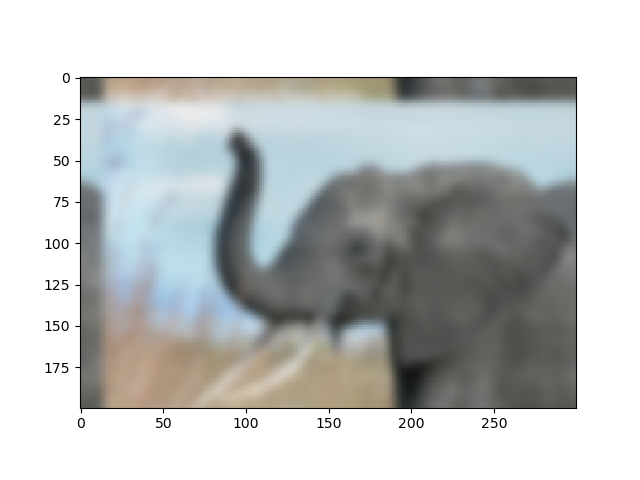
Here we will blur the original images using the Gaussian filter and see how to control the level of smoothness using the sigma parameter.

from scipy import ndimage,misc
import matplotlib.pyplot as plt

face = scipy.misc.face(gray=True)
blurred_face = ndimage.gaussian_filter(face, sigma=3)
very_blurred = ndimage.gaussian_filter(face, sigma=5)

plt.figure(figsize=(9, 3))
plt.subplot(131)
plt.imshow(face, cmap=plt.cm.gray)
plt.axis('off')
plt.subplot(132)
plt.imshow(very_blurred, cmap=plt.cm.gray)
plt.axis('off')
plt.subplot(133)
plt.imshow(blurred_face, cmap=plt.cm.gray)
plt.axis('off')


plt.subplots_adjust(wspace=0, hspace=0., top=0.99, bottom=0.01,
                    left=0.01, right=0.99)

plt.show()

Output:

The first image is the original image followed by the blurred images with different sigma values.

Sharpening images

Here we will blur the image using the Gaussian method mentioned above and then sharpen the image by adding intensity to each pixel of the blurred image.

import scipy
from scipy import ndimage
import matplotlib.pyplot as plt

f = scipy.misc.face(gray=True).astype(float)
blurred_f = ndimage.gaussian_filter(f, 3)

filter_blurred_f = ndimage.gaussian_filter(blurred_f, 1)

alpha = 30
sharpened = blurred_f + alpha * (blurred_f - filter_blurred_f)

plt.figure(figsize=(12, 4))

plt.subplot(131)
plt.imshow(f, cmap=plt.cm.gray)
plt.axis('off')
plt.subplot(132)
plt.imshow(blurred_f, cmap=plt.cm.gray)
plt.axis('off')
plt.subplot(133)
plt.imshow(sharpened, cmap=plt.cm.gray)
plt.axis('off')

plt.tight_layout()
plt.show()

Output:

Edge detection

Edge detection includes a variety of mathematical methods that aim at identifying points in a digital image at which the image brightness changes sharply or, more formally, has discontinuities. The points at which image brightness changes sharply are typically organized into a set of curved line segments termed edges.

Here is an example where we make a square figure and then find its edges:

mport numpy as np
from scipy import ndimage
import matplotlib.pyplot as plt

im = np.zeros((256, 256))
im = 1

im = ndimage.rotate(im, 15, mode='constant')
im = ndimage.gaussian_filter(im, 8)

sx = ndimage.sobel(im, axis=0, mode='constant')
sy = ndimage.sobel(im, axis=1, mode='constant')
sob = np.hypot(sx, sy)

plt.figure(figsize=(9,5))
plt.subplot(141)
plt.imshow(im)
plt.axis('off')
plt.title('square', fontsize=20)
plt.subplot(142)
plt.imshow(sob)
plt.axis('off')
plt.title('Sobel filter', fontsize=20)
plt.show()

Output:

Преобразование Fourier

Анализ Fourier помогает нам выразить функцию, как сумму периодических компонентов и восстановить сигнал из этих компонентов.

Давайте посмотрим на простой пример преобразования Fourier. Мы будем строить сумму двух синусов:

# Import Fast Fourier Transformation requirements
from scipy.fftpack import fft
import numpy as np

# Number of sample points
N = 600

# sample spacing
T = 1.0 / 800.0
x = np.linspace(0.0, N*T, N)
y = np.sin(50.0 * 2.0*np.pi*x) + 0.5*np.sin(80.0 * 2.0*np.pi*x)
yf = fft(y)
xf = np.linspace(0.0, 1.0/(2.0*T), N//2)

# matplotlib for plotting purposes
import matplotlib.pyplot as plt
plt.plot(xf, 2.0/N * np.abs(yf[0:N//2]))
plt.grid()
plt.show()

Mass:

Return the specified unit in kg (e.g.
returns )

Example

from scipy import constants

print(constants.gram)        #0.001print(constants.metric_ton)  #1000.0
print(constants.grain)       #6.479891e-05
print(constants.lb)          #0.45359236999999997
print(constants.pound)       #0.45359236999999997
print(constants.oz)          #0.028349523124999998
print(constants.ounce)       #0.028349523124999998
print(constants.stone)       #6.3502931799999995
print(constants.long_ton)    #1016.0469088
print(constants.short_ton)   #907.1847399999999
print(constants.troy_ounce)  #0.031103476799999998
print(constants.troy_pound)  #0.37324172159999996
print(constants.carat)       #0.0002
print(constants.atomic_mass) #1.66053904e-27print(constants.m_u)         #1.66053904e-27
print(constants.u)           #1.66053904e-27

1.6.9. Signal processing: scipy.signal¶

Tip

is for typical signal processing: 1D,
regularly-sampled signals.

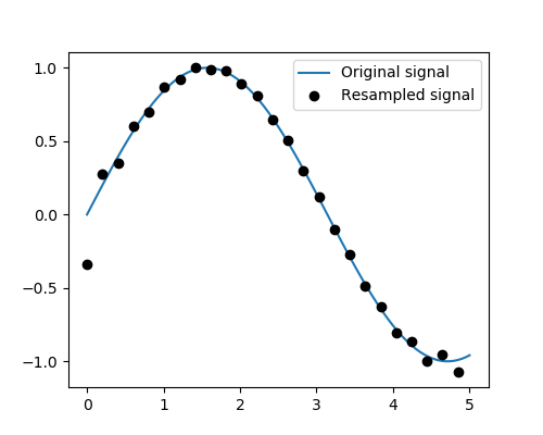
Resampling : resample a signal to n
points using FFT.

>>> t = np.linspace(, 5, 100)
>>> x = np.sin(t)

>>> from scipy import signal
>>> x_resampled = signal.resample(x, 25)

>>> plt.plot(t, x) 

>>> plt.plot(t, x_resampled, 'ko') 

Tip

Notice how on the side of the window the resampling is less accurate
and has a rippling effect.

This resampling is different from the provided by as it
only applies to regularly sampled data.

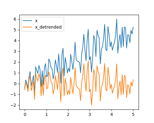
Detrending : remove linear trend from signal:

>>> t = np.linspace(, 5, 100)
>>> x = t + np.random.normal(size=100)

>>> from scipy import signal
>>> x_detrended = signal.detrend(x)

>>> plt.plot(t, x) 

>>> plt.plot(t, x_detrended) 

Filtering:
For non-linear filtering, has filtering (median
filter , Wiener ),
but we will discuss this in the image section.

Tip

also has a full-blown set of tools for the design
of linear filter (finite and infinite response filters), but this is
out of the scope of this tutorial.

Spectral analysis:
compute a spectrogram –frequency
spectrums over consecutive time windows–, while
comptes a power spectrum density (PSD).

Составные части

Пакет SciPy лежит в основе научных вычислительных возможностей Python. Доступные подпакеты включают:

• кластер : иерархическая кластеризация , векторное квантование , K-средних
• константы : физические константы и коэффициенты преобразования
• fft : алгоритмы дискретного преобразования Фурье
• fftpack : устаревший интерфейс для дискретных преобразований Фурье
• интегрировать : процедуры численного интегрирования
• интерполировать : инструменты интерполяции
• io : ввод и вывод данных
• linalg : процедуры линейной алгебры
• разное : разные утилиты (например, примеры изображений)
• ndimage : различные функции для обработки многомерных изображений
• ODR: классы и алгоритмы ортогональной дистанционной регрессии
• optimize : алгоритмы оптимизации, включая линейное программирование
• signal : инструменты обработки сигналов
• sparse : разреженные матрицы и связанные алгоритмы
• пространственные : алгоритмы для пространственных структур, таких как деревья kd , ближайшие соседи, выпуклые оболочки и т. д.
• special : специальные функции
• stats : статистические функции
• weave : инструмент для написания кода C / C ++ в виде многострочных строк Python (теперь не рекомендуется в пользу Cython )

Снимок, показывающий исходный код SciPy ndimage

Что такое Python?

По состоянию на 2020 год Python является одним из самых популярных языков программирования, который входит в ТОП-10, а также считается одним из наиболее простых для обучения программированию. Если вы только начинаете изучать основы программирования, то Python для вас — лучший выбор.

На нашем сайте вы сможете пройти полный курс по языку программирования Python (читается как Пайтон или Питон) онлайн абсолютно . Курс будет полезен как для начинающих веб-разработчиков, так и для профессионалов как справочное пособие для дальнейшей работы.

Python произносится как Пайтон, но в русскоязычной среде часто произносят как «Питон», что в общем-то не является большой ошибкой. Каждый может произносить название Python как хочет или как ему удобно.

Python используется для:

• веб-разработка (на стороне сервера);
• разработка программного обеспечения;
• математика;
• системные скрипты.

Что может делать Python?

• Python может использоваться на сервере для создания веб-приложений.
• Python может использоваться вместе с программным обеспечением для создания рабочих процессов.
• Python может подключаться к системам баз данных. Он также может читать и изменять файлы.
• Python может использоваться для обработки больших данных и выполнения сложной математики.
• Python можно использовать для быстрого прототипирования или для разработки программного обеспечения, готового к производству.

Почему надо изучать Python?

• Python работает на разных платформах (Windows, Mac, Linux, Raspberry Pi и т.д.).
• Python имеет простой синтаксис, похожий на обычный английский язык.
• Python имеет синтаксис, который позволяет разработчикам писать программы с меньшим количеством строк, чем некоторые другие языки программирования.
• Python работает в системе интерпретатора, что означает, что код может быть выполнен, как только он написан. Это означает, что прототипирование может быть очень быстрым.
• Python может рассматриваться как процедурный, объектно-ориентированный или функциональный.

Что нужно знать про Python?

• Самая последняя основная версия Python — это Python 3, который мы будем использовать в этом учебнике. Тем не менее, Python 2, хотя и не обновляется ничем, кроме обновлений безопасности, все ещё довольно популярен.

• Python был разработан для удобства чтения и имеет некоторые сходства с английским языком с влиянием математики.
• Python использует новые строки для завершения команды, в отличие от других языков программирования, которые часто используют точки с запятой или круглые скобки.
• Python использует отступы, используя пробелы для определения области видимости, такие как область действия циклов, функций и классов. Другие языки программирования часто используют фигурные скобки для этой цели.

Performing calculations on Polynomials with Python SciPy

The sub-module of the SciPy library is used to perform manipulations on 1-d polynomials. It accepts coefficients as input and forms the polynomial objects.

Let’s understand the poly1d sub-module with the help of an example.

Example:

from numpy import poly1d

# Creation of a polynomial object using coefficients as inputs through poly1d
poly_input = poly1d()

print(poly_input)

# Performing integration for value = 4
print("\nIntegration of the input polynomial: \n")
print(poly_input.integ(k=3))

# Performing derivation
print("\nDerivation of the input polynomial: \n")
print(poly_input.deriv())

In the above snippet of code, is used to accept the coefficients of the polynomial.

Further, is used to find the integration of the input polynomial around the input scalar value. The function is used to calculate the derivation of the input polynomial.

Output:

   3     2
2 x + 4 x + 6 x + 8

Integration of the input polynomial: 

     4         3     2
0.5 x + 1.333 x + 3 x + 8 x + 3

Derivation of the input polynomial: 

   2
6 x + 8 x + 6

Discrete Fourier Transform – scipy.fftpack

• DFT is a mathematical technique which is used in converting spatial data into frequency data.
• FFT (Fast Fourier Transformation) is an algorithm for computing DFT
• FFT is applied to a multidimensional array.
• Frequency defines the number of signal or wavelength in particular time period.

Example: Take a wave and show using Matplotlib library. we take simple periodic function example of sin(20 × 2πt)

%matplotlib inline
from matplotlib import pyplot as plt
import numpy as np 

#Frequency in terms of Hertz
fre  = 5 
#Sample rate
fre_samp = 50
t = np.linspace(0, 2, 2 * fre_samp, endpoint = False )
a = np.sin(fre  * 2 * np.pi * t)
figure, axis = plt.subplots()
axis.plot(t, a)
axis.set_xlabel ('Time (s)')
axis.set_ylabel ('Signal amplitude')
plt.show()

Output:

You can see this. Frequency is 5 Hz and its signal repeats in 1/5 seconds – it’s call as a particular time period.

Now let us use this sinusoid wave with the help of DFT application.

from scipy import fftpack

A = fftpack.fft(a)
frequency = fftpack.fftfreq(len(a)) * fre_samp
figure, axis = plt.subplots()

axis.stem(frequency, np.abs(A))
axis.set_xlabel('Frequency in Hz')
axis.set_ylabel('Frequency Spectrum Magnitude')
axis.set_xlim(-fre_samp / 2, fre_samp/ 2)
axis.set_ylim(-5, 110)
plt.show()

Output:

• You can clearly see that output is a one-dimensional array.
• Input containing complex values are zero except two points.
• In DFT example we visualize the magnitude of the signal.

Проверка на нормальность в Scipy

Нормальный закон распределения является простым и удобным для дальнейшего исследования. Чтобы проверить имеет ли тот или иной атрибут нормальное распределение, можно воспользоваться двумя критериями Python-библиотеки с модулем . Модуль   поддерживает большой диапазон статистических функций, полный перечень которых представлен в официальной документации.

В основе проверки на “нормальность” лежит проверка гипотез. Нулевая гипотеза – данные распределены нормально, альтернативная гипотеза – данные не имеют нормального распределения.

Проведем первый критерий Шапиро-Уилк [], возвращающий значение вычисленной статистики и p-значение. В качестве критического значения в большинстве случаев берется 0.05. При p-значении меньше 0.05 мы вынуждены отклонить нулевую гипотезу.

Проверим распределение атрибута Rings, количество колец:

import scipy

stat, p = scipy.stats.shapiro(data) # тест Шапиро-Уилк
print('Statistics=%.3f, p-value=%.3f' % (stat, p))

alpha = 0.05
if p > alpha:
    print('Принять гипотезу о нормальности')
else:
    print('Отклонить гипотезу о нормальности')

В результате мы получили низкое p-значение и, следовательно, отклоняем нулевую гипотезу:

Statistics=0.931, p-value=0.000
Отклонить гипотезу о нормальности

Второй тест по критерию согласия Пирсона [], который тоже возвращает соответствующее значение статистики и p-значение:

stat, p = scipy.stats.normaltest(data) # Критерий согласия Пирсона
print('Statistics=%.3f, p-value=%.3f' % (stat, p))

alpha = 0.05
if p > alpha:
    print('Принять гипотезу о нормальности')
else:
    print('Отклонить гипотезу о нормальности')

Этот критерий также отвергает нулевую гипотезу о нормальности распределения колец у моллюсков, так как p-значение меньше 0.05:

Statistics=242.159, p-value=0.000
Отклонить гипотезу о нормальности

Линейная алгебра с Python SciPy

Линейная алгебра представляет линейные уравнения и представляет их с помощью матриц.

Подмодуль библиотеки SciPy используется для выполнения всех функций, связанных с линейными уравнениями. Он преобразует объект в 2-D массив NumPy, а затем выполняет задачу.

1. Решение системы уравнений

Давайте разберемся в работе подмодуля linalg вместе с линейными уравнениями с помощью примера:

4x+3y=12 3x+4y=18

Рассмотрим приведенные выше линейные уравнения. Давайте решим уравнения с помощью функции .

from scipy import linalg
import numpy
X=numpy.array(,])
Y=numpy.array(,])
print(linalg.solve(X,Y))
X.dot(linalg.solve(X,Y))-Y

В приведенном выше фрагменте кода мы передали коэффициенты и постоянные значения, присутствующие во входных уравнениях, через функцию numpy.array ().

Далее, решает линейные уравнения и отображает значение x и y, которое работает для этого конкретного уравнения. используется для проверки вывода уравнений.

Выход:

 ]
array(,
       ])

массив(, ]) гарантирует, что линейные уравнения были правильно решены.

] : Это значения x и y, используемые для решения линейных уравнений.

2. Нахождение детерминант матриц

Метод используется для поиска определителя входной матрицы.

Пример :

from scipy import linalg
import numpy
determinant=numpy.array(,])
linalg.det(determinant)

Выход:

8.0

3. Вычисление обратной матрицы

Метод используется для вычисления обратной входной матрицы.

Пример:

from scipy import linalg
import numpy
inverse=numpy.array(,])
linalg.inv(inverse)

Выход:

array(,
       ])